Class 10 – IT – Code 402 – Electronic Spreadsheet Practical File Questions with Solution

Find Class 10 Information Technology Code 402 Practical or Project File Questions with Complete Solution for Teachers and Students to Make your Project or Practical File from Digital Documentation (Advanced) including Applying Styles in a Document, Adding Graphics in a Document, Working with Templates, Using a Table of Contents and Using Mail Merge.
Electronic Spreadsheet (Advanced) including Analysing Data in a Spreadsheet, Linking Data and Spreadsheets, Sharing and Reviewing a Spreadsheet and Using Macros in a Spreadsheet.
Database Management System including Concepts of Database Management System, Creating and Using Tables, Performing Operations on Tables, Retrieving Data using Quesries and Working with Forms and Reports.
Web Applications and Security including Creating a Blog using Online or Offline Editor, Internet shopping for Online Shopping, Safety measures for Online Transactions, Common Hazards and Workplace and Case Study based.

Unit II – Electronic Spreadsheet (Advanced)

Analysing Data in Spreadsheet

Practical 1 (Source: Kips)

ABC is a furniture store that has branches across the city. The finance team wants to consolidate the sales of a few products from the top three branches in the current financial year. The data maintained by the three branches is shown below:

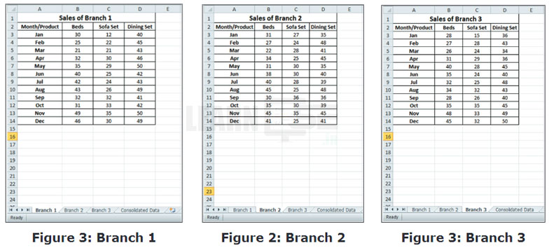
Consolidate the data of these sheets in the fourth sheet ‘Consolidated Data’.

For MS Excel

For Calc (Open Office)

« Enter the headings and names of cars in the fourth sheet “Consolidated Data’. « Click on the Data tab and select Consolidate, The Consolidate dialog box appears. « In the Function drop-down list, select a function. For example, to get the sum of data of both the worksheets, select the Sum function. « Click inside the Reference text box. Then, go to sheet 1 (Branch 1), and drag the mouse to select the first source data range on the sheet. « Click on the Add button. The selected range is added in the All References list box. « Similarly, choose data range from sheet 2 (Branch 2) and sheet 3 (Branch 3) and add them in the corresponding All References list boxes. « Now, click on OK. You will get the consolidated data of all the sheets in the ‘Consolidated Data’ sheet.

« On sheet 3 (Branch 3), click on the Data menu and select the Consolidate option. « The Consolidate dialog box appears. Here, in the Function drop-down list, select a function. For example, to get the sum of the data available on both the worksheets, select the Sum function. « Click inside the Source data ranges text box. Then, go to sheet 1 (Branch 1), and drag the mouse to select the first source data range on the sheet. « Click on the Add button in the dialog box. The selected range is added in the Consolidation ranges list box. « Similarly, add data range from sheet 2 (Branch 2) and sheet 3 (Branch 3) and add it in the Consolidation ranges list box. « Click in the Copy results to list box. Go to sheet 3 (Branch 3) and select first cell of the target range instead of selecting the entire range. « Now, click on OK. You will get the consolidated data of all the sheets in the ‘Consolidated Data’ sheet.

Practical 2 (Source: Kips)

A car manufacturing company is planning its goals about the sales of various models of cars in the fourth quarter, so as to obtain 80% sales for the year. The percentage of sales in three quarters is shown in the given table.

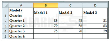
Find out how much sales is required by the company to obtain their target.

For MS Excel:

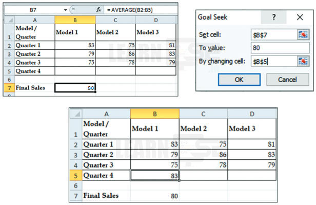
• Type ‘Quarter 4′ in cell A5.
• Type ‘Final Sales’ in cell A7 and enter the formula AVERAGE(B2:B5).
• Now, select the cell B5 and click on the Data tab.
• From tne Data Tools group, click on the What-If Analysis drop-down button and select the Goal Seek option.
• The Goal Seek dialog box appears.
• In the Goal Seek dialog box, click inside the Set cell box.
• Now, click on the cell B7. Its value will be automatically entered in the Set cell box.
• In the To value box, enter 80 (targeted value).
• Now, click inside the By changing cell box and select cell B5. Its value will be automatically entered in the By changing cell box.
• Click on OK. The Goal Seek tool will calculate the estimated value that appears in the cell B5.
• Similarly, do the same for the Model 2 and Model 3 also. You will get the estimated values for them too.

For Calc:

• Type ‘Quarter 4′ in cell A5 and 0 in cell B5.
• Type ‘Final Sales’ in cell A7 and enter the formula AVERAGE(B2:B5).
• Choose the Tools menu > Goal Seek option.
• The Goal Seek dialog box opens. Define the values in the following fields, as per your requirement.
  • Formula cell: It contains the reference of the cell that has a formula. For example, click on the Formula cell field and select the cell B7 in the sheet, which has the formula.
  • Target value: It contains the value that you want to achieve as new result. So, Enter the desired result of the formula in the Target value field, which here is 80.
  • Variable cell: It contains the value that you want to adjust in order to reach the target. For this, click on the Variable cell field and select cell B5; whose value is to be changed.
• Click on OK and you will get a pop-up displaying the result. Click on Yes to insert it in cell B5 and notice the output.
• Similarly, do the same for the Model 2 and Model 3 also. You will get the estimated values for them too.

Linking Data in Spreadsheets

Practical 1 (Source: Kips)

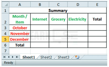
Anjali wants to summarise and compare the total expenditure of her household for the months of October, November and December. She has maintained this dats in three worksheets as shown below:

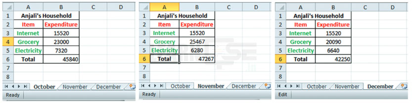
Help Anjali to summarise the tots! expenditure item-wise as well as month-wise in another workbook.

For MS Excel:

• Create another workbook (named as Book2) with the Sheet1 (Summary) as shown here.
  
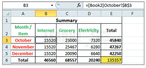
• In the cell B3, type “=” sign, but do not press the Enter key.
• Now, navigate to the workbook that contains the data for the month of October.
• Click on cell B3 in the October sheet and press Enter.
• The reference to this cell will be created in the Book2 and the value will be reflected in the corresponding cell.
• Similarly, create references for the other items as well in the Book2.
• Now, you can calculate the total expenditure item-wise as well as month-wise by applying the Sum formula.
• Observe the Sheet1 (Summary sheet) for the output.

For Calc:

• Open the spreadsheet and enter the data as shown.
• Open a new spreadsheet in which the link is to be created.
• Click on cell B3 where the formula is to be entered and type =Sum ( .
• With the opening parenthesis, click on the Windows menu and select a sheet to switch into. Then, select the cell address. For example, select Untitled1, October, and cell B3.
• Then, press the Ctrl key and switch into the next sheet to get the reference, and so on.
• Once completed, switch back to the original sheet and enter the close parentnesis ‘)’ .
• Press the Enter key. You will get the resultant value in the cell.
• After linking, to calculate the total expenditure item-wise as well as month-wise by applying the Sum formula.
• Observe the Untitled 2, Sheet1 (Summary sheet) for the output.

Practical 2 (Source: Kips)

Create a worksheet in Excel and insert a hyperlink in the same worksheet that leads to a specified location.

For MS Excel:

• Create a new worksheet in Excel.
• Click on the cell where you want to insert a hyperlink.
• Choose Insert > Hyperlink.
• The Insert Hyperlink dialog box opens.
• Select the Place in This Document category in the dialog box.
• Choose the following options to create a hyperlink at a particular place in the current workbook:
  • In the Text to display textbox, type the text that is to be displayed as the linked text.
    
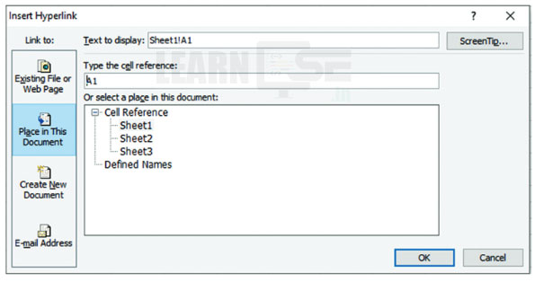
  • In the Type the cell reference textbox, enter the reference(s) of the cell(s) to be linked.
  • In the Or select a place in the document section, choose from the list of sheets under Cell Reference or Defined Names to select the area to be linked.
• Click on OK to insert the link.

For Calc:

To insert a hyperlink in a spreadsheet, follow these steps:

• Bring the mouse pointer at the point where you want to insert a hyperlink. Or
• Select the text that you want fo put as a hyperlink.
• Choose Insert > Hyperlink from the menu bar.
• The Hyperlink dialog box opens. It contains the categories, Internet, Mail, Document, and New Document.
• Select the required category to create hyperlink. For example, select Document in the Hyperlink dialog box and enter tne document path.
• Click on OK to insert the link.

Sharing and Reviewing a Spreadsheet – Updated soon

Practical 1 (Source: Kips)

Practical 2 (Source: Kips)

Using Macros in a Spreadsheet – Updated soon

Practical 1 (Source: Kips)

Practical 2 (Source: Kips)