
Unit 2 – Electronic Spreadsheet (Advanced)
What is Spreadsheet?
It is program (software) that is used to do calculation and store the records. It allows you to store, organize, calculate and manipulate the saved or available data in a tabular format. It consists rows and columns. It provides inbuilt features and data analysis tools that make it easier to work with the large amount of data.
Some important points to learn about Spreadsheet Program
- An Excel File is also known as workbook or spreadsheet program.
- A sheet of an excel file is known as worksheet.
- A combination of worksheets is known as workbook.
- There are 3 worksheets available in Excel by default.
- By default, the name of Excel file is Book1.
- The smallest unit of MS Excel file is a cell.
- A cell is an intersection of a row and column.
- Horizontal series of cells is known as row.
- Vertical series of cells is known as column.
- In spreadsheet A, B, C, D…… termed as column name.
- In spreadsheet 1, 2, 3, 4…… termed as row number.
- Section A, B, C, D…..are known as column header.
- Section 1, 2, 3, 4…..are known as row header.
- Home, Insert, View => Tabs
- Bold, Italic, Underline, Font size => Functions or Tools
- Clipboard, Paragraph… => Groups
- Topmost bar of an Excel file is known as Title Bar.
- Last column name – XFD
- Last row number / Total no of rows – 10,48,576
- Total no of columns – 16,384
- Total no of sheets – 255
- Total no of characters in a cell – 32,767
- Some popular spreadsheet software are:
- Microsoft Excel – Desktop based
- Google Sheets (part of Google docs) – Internet base
- LibreOffice
- Apache OpenOffice Calc
5 features of an Excel program
- Functions and Formulas: In MS Excel, there are many built-in functions and formulas which are used to perform action over the sheet and calculation respectively. Some calculation based formulas are: Sum, Average, Max etc.
- Formatting options: These options are used to enhance the appearance of stored data.
- Auto-Calculation: The data is automatically recalculated in the whole worksheet if any changes are made in different cells or one cell.
- Fast Searching: In this a user can search data fast as well as replace or edit instantly.
- Sort and Filter Tool: These tools are used to arrange data in systematic way. We use sort to arrange in alphabetical order and filter is used to search or find any specific data.
Some Important Basic Shortcut Keys for Excel
| To open an existing file | CTRL + O |
| To save a file | CTRL + S |
| To create a new file | CTRL + N |
| To close a file (Excel sheet) | CTRL + W |
| To close an application (Excel file) | ALT + F4 |
| To print | CTRL + P |
| To undo the changes | CTRL + Z |
| To move to previos stage (Redo) | CTRL + Y |
| To select any tool from ribbon | ALT + DESIRED CHARACTER(S) |
| To open save as dialog box | F12 |
| To open the help pane | F1 |
| To search in spreadsheet | CTRL + F |
Some Important Advanced Shortcut Keys for Excel
| To move to the NEXT sheet | CTRL + PAGE DOWN KEY (Pg Dn) |
| To move to the previous sheet | CTRL + PAGE UP KEY (Pg Up) |
| To minimize the workbook window | CTRL + F9 |
| To create a new worksheet | SHIFT + F11 |
| To copy the above cell data | CTRL + D |
| To repeat commands | F4 |
| To get total of adjacent cells | ALT + Equal Key (=); i.e. Autosum |
| To display the insert dialog box | CTRL + SHIFT + EQUAL KEY |
| To apply filter | CTRL + SHIFT + L |
| To open Visual Basic Prompt (Window) | ALT + F11 |
| To insert a new comment in a cell | SHIFT + F2 |
CHAPTER 1 – ANALYSING DATA IN A SPREADSHEET
Data Consolidation
Data consolidation means that you can combine all the data of different worksheets in a single worksheet.
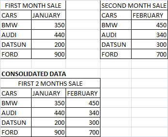
First Month Sale and Second Month Sale Data Consolidated as First 2 Month Sale in another sheet.
Steps to use or Create Consolidate option to Consolidate Data
STEPS: DATA TAB > DATA TOOLS GROUP > CONSOLIDATE OPTION
- Step1: Create tables in different sheets with same parameters (fields).
- Step2: Move to the particular sheet where you want to create a consolidated table.
- Step3: Click on Consolidate option after selecting desired cell range.
- Step4: Add cell references of previously created tables in reference text box. Then click on Add button. Add all cell references and select function as SUM.
- Step5: Click on OK button. Consolidated data will be visible in the sheet that you selected first.
Scenario Manager
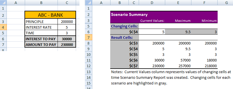
It is an important tool of MS Excel, that enables you to manage and view data from different input values. For example, if you want to calculate the effect of different interest rates on an investment, you could add a scenario for each interest rate, and quickly view the results.
Steps to apply Scenario Manager (To find simple interest on maximum and minimum rate)
STEPS: DATA TAB > DATA TOOLS GROUP > WHAT-IF ANALYSIS TOOL > SCENARIO MANAGER OPTION
- Step 1: Insert data in a table to create different scenarios
- Step 2: Click on Scenario Manager option in the What-If analysis tool of Data tab. A Scenario Manager dialog box will appear.
- Step 3: Click on Add, Define scenario name and select the cell or cell range that you want to change and Click on Ok.
- Step 4: Now select scenario and click on show button to see the new scenario or click on Summary button to show all scenarios.
Goal Seek
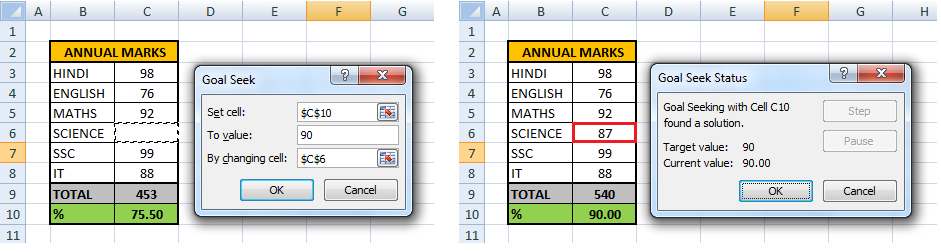
It is a useful data analysis tool of MS Excel software. It is used to set a goal to find the optimum (correct) value for one or more target variables, given with the certain conditions. Simply it helps you obtain the input value that results in the target value that you want.
Steps to apply Goal Seek Tool
STEPS: DATA TAB > DATA TOOLS GROUP > WHAT-IF ANALYSIS TOOL > GOAL SEEK OPTION
- Step 1: Create a table to find optimum value.
- Step 2: Click on Goal Seek option in the What-If analysis tool of Data tab. A Goal Seek dialog box will appear.
- Step 3: Define target cell address in ‘Set Cell’, Target value in ‘To value’ and Input variable address in ‘By changing cell’ then click on OK
- Value will be visible as per the target value.
Solver
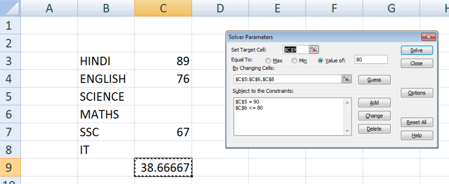
Solver is another What-if Analysis tool. It follows the Goal Seek method to solve the equations but more elaborately. The only difference between Goal Seek and Solver is that the Solver deals with equations with multiple unknown variables. It is the elaborate form of Goal Seek tool.
Steps to Enable or Disable Solver Tool
DATA TAB > ANALYSIS GROUP > SOLVER OPTION
- Step 1: Click on file button
- Step 2: Click on “Excel Options / Options” Option
- Step 3: Click on add-ins option
- Step 4: Click on go button under manage option
- Step 5: Check “solver add-in” And click on ok button, solver tool will be installed
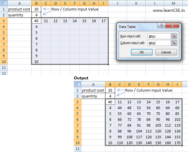
Data Table
It is a way to see different results by altering an input cell in your formula. Instead of using or creating different scenarios, you can create a data table quickly try out the different values for the formula.
CHAPTER 2 – LINKING DATA AND SPREADSHEETS
Difference between the Absolute and Relative hyperlinks
The Absolute Hyperlink is a hyperlink that contains the full address of the destination file or webpage.
Example: https://learncse.in/about-us/ or D:\Entrance\New Folder\winter.jpg
The Relative Hyperlink contains a partial address, which is relative to the address of the destination file.
Example: If you have saved a worksheet/workbook “abc.xlsx” and an image file “winter.jpg” in D: drive. To create a relative hyperlink of the image file to the workbook, the relative path will be “\winter.jpg”.
Different types of hyperlinks that can be applied in spreadsheets
- Cell Reference Hyperlinks: These hyperlinks allow you to link to a specific cell within the same spreadsheet or a different spreadsheet in the same workbook.
- Sheet Hyperlinks: These hyperlinks enable you to link to a specific sheet within the same workbook.
- External File (Document/Picture) Hyperlinks: You can create hyperlinks to files stored on your local memory or network.
- Webpage Hyperlinks: Hyperlinks can also link to external webpages.
- Email Hyperlinks: You can create hyperlinks to compose emails. When clicked, these hyperlinks open the default email client with the recipient’s email address pre-filled.
- Formula Hyperlinks: You can create hyperlinks based on certain conditions or criteria within your spreadsheet.
Why do you link the spreadsheets data?
Linking spreadsheet data enables you to keep the information updated without editing in multiple locations, every time the data changes. The ability to create links eliminate the need of having identical data entered and updated in multiple sheets. This saves time, reduces errors and improves data integrity. It is a quick way to get the data from one worksheet to another by using the ‘copy and paste’ method.
Write the steps to fetch data from “B3 cell of Book1.xlsx” into “B3 cell of Book2.xlsx”.
- Step 1: Open Book1.xlsx and Book2.xlsx
- Step 2: Click on B3 cell of Book2.xlsx and press = (equal) sign.
- Step 3: Click on View Tab and Select Switch Windows option and choose Book1.
- Step 4: Select B3 of Book1.xlsx and press Enter.
='[Book1.xlsx]Sheet2′!B3
How can you import the data from external data sources in excel?
To import the data from external data sources, the steps are following:
- Step 1: Click on Data Tab.
- Step 2: Select Desired file source (Eg: From Access) option in Get External Data Group.
- Step 3: “Select Data Source” dialog box will appear. Select the desired file by moving to the particular location of stored file.
- Step 4: Click on Open. The content of the source file will be fetched into destination file.
CHAPTER 3 – SHARING AND REVIEWING A SPREADSHEET
What are comments?
In spreadsheet, comments help in providing some extra information on the data stored in a cell. They play an important role to add some facts, tips or feedback for the user.
- Steps to Insert New Comment in Excel
- Review Tab > Comments Group > New Comment Option
- Steps to Edit or Delete Comments
- Review Tab > Comments Group > Delete option / Edit Comment option
Why are track changes needed?
Sometimes, you may be required to record the changes done by you or the other users in a spreadsheet to review later. It enables you to keep a track of the changes done by you or the other users such as addition, deletion, content alteration, formatting and makes the changes visible in order to ease the review process.
- Not all changes are recorded likewise, the changes in the alignment of the cell content.
Steps to add Compare and Merge workbooks option
The Compare and Merge Workbooks option is not available in Excel, by default. It can be added to the Quick access toolbar using the following steps:
- Step 1: Click on File button and choose Excel options. The Excel options dialog box will appear.
- Step 2: Select Quick Access Toolbar or Customize option.
- Step 3: Under Choose commands from, click on the drop-down menu and select All commands option.
- Step 4: Find and Select Compare and Merge Workbooks option.
- Step 5: Click to Add to add it to the Quick Access Toolbar.
- Step 6: Click on OK.
Why do you compare and merge spreadsheets?
When multiple users collaborate on the same shared workbook, you can use the Compare and Merge Workbooks command to view all of their changes at once and address them by accepting or rejecting them.
Each person you collaborate with must save a copy of the shared workbook using a unique file name that differs from the original.
For example, if the original file name is LEARNCSE, your collaborators could use the files names LEARNCSE—Mohit’s Changes or Samit-LEARNCSE.
- You can only merge copies of the same shared workbook. All of the copies you plan to merge should be located in the same folder.
How can a group of people work on the same excel spreadsheet simultaneously in Excel 2007/2013?
In Microsoft Office Excel 2007
- Step 1: Click the Review tab.
- Step 2: Click Share Workbook in the Changes group.
- Step 3: On the Editing tab, click to select the Allow changes by more than one user at the same time. This also allows workbook merging check box, and then click OK.
- Step 4: In the Save As dialog box, save the shared workbook on a network location where other users can gain access to it.
In Microsoft Office Excel 2013
- Step 1: On the Tools menu, click Share Workbook, and then click the Editing tab.
- Step 2: Click to select the Allow changes by more than one user at the same time check box, and then click OK. Save the workbook when you are prompted.
- Step 3: On the File menu, click Save As, and then save the shared workbook on a network location where other users can gain access to it.
CHAPTER 4 – USING MACROS IN A SPREADSHEET
What is a macro in Excel?
A macro is like an algorithm or a set of actions that we can use or run multiple times. A macro helps in automating or repeating tasks by recording or storing our input sequences like mouse strokes or keyboard presses. Once this input is stored, it makes up a macro which is open to any possible changes.
Steps to record a macro.
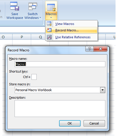
- Step 1: In the Macros group on the View tab, click Macro.
- Step 2: Select Record Macro option.
- Step 3: Write Macro name and assign shortcut key. Select desired option to store macro and a description (optional) in the Description box, and then click OK to start recording.
- Step 4: Perform the actions you want to automate, such as entering or filling down a column of data.
- Step 5: On the View tab or status bas, click Stop Recording.
What is macro writing?
Excel Macro is a record and playback tool that simply records your Excel steps and the macro will play it back as many times as you want. VBA Macros save time as they automate repetitive tasks. It is a piece of programming code that runs in an Excel environment but you don’t need to be a coder to program macros.
Function
A function is a set of code that executed on function calling. When you call a function , it gets invoked and returns result as per the data/code. To define a macro as function, use the keyword Function. Each function has a name and may have parameters whose values you pass when you call the function.
Macro functions can be written to behave as regular functions by writing an Add-in.
Syntax:
Function Function_Name ()
Function_Name = Result //Body of Function
End Function
Example.1: Code to use macro as a function. (Function to add)
Function Total()
Total = 10 + 20
End Function

Output: 30
(By writing =total() in a cell of MS Excel)
Example 2: Code without passing arguments to a macro
Sub Button1_Click()
MsgBox Total
End Sub
------------------
Function Total ()
Total = 10
MsgBox Total
End Function
Example 3: Code with passing arguments to a macro
Sub Button1_Click()
MsgBox Total(x)
End Sub
------------------
Function Total(x)
x = 10
MsgBox x
End Function
Here, Button1_Click() is a command button. MsgBox Total(x) is a function calling through which an integer value can be passed as an argument. Function Total(x) …… End Function is the body of the function.
A macro acts as a function. You can pass arguments (values/parameters) to a macro when you call it. To allow a macro to accept a value, simply type a name for that value between the parenthesis at the top of the macro.
Example 4: Passing arguments to a macro by Reference – means you are referring to the original value.
Sub Button1_Click()
Dim x As Integer
x = 10
MsgBox Total(x)
MsgBox x
End Sub
---------------------------
Function Total(ByRef x As Integer)
x = x * 5
Total = x
End Function
Example 5: Passing arguments to a macro by Value – means you are passing a copy of the value to the function while calling it.
Sub Button1_Click()
Dim x As Integer
x = 10
MsgBox Total(x)
MsgBox x
End Sub
---------------------------
Function Total(ByVal x As Integer)
x = x * 5
Total = x
End Function
Built-in Function to calculate age:
=(TODAY()-DOB_CELL_ADD)/365
=INT((TODAY()-DOB_CELL_ADD)/365)
Macro allows you to create custom functions using VBA, called the User Defined Functions, which can be used in the same way as you use the SUM() function or other built-in Excel functions.
Follow these steps to create a function that works as a built-in Excel function to find Age from starting date to end date:
- Step 1: Open a new excel workbook.
- Step 2: Get into VBA (Visual Basic for Applications) by pressing Alt + F11.
- Step 3: Click on Insert > Module option, to insert a new module.
- Step 4: Write the following code to create a function to calculate the age of a person using the start and end date.
Function AgeInYears(start_date As Variant, end_date As Variant)
AgeInYears = Year(end_date) – Year(start_date) – Abs (DateSerial(Year(end_date), Month (start_date), Day(start_date)) > DateValue(end_date))
End Function- Step 5: Save the function and move to the excel file by switching application or press Alt + F11 or press Alt + Q to exit the VBA.
- Step 6: Open MS Excel and use the function as:
=AgeInYears(“10-Dec-2003”, “4-Dec-2020”)- Step 7: Press Enter key.
Steps to work on user defined function as built-in functions
- Step 1: Press Shift + F3 or Click on Formulas Tab > Insert Function. The Insert Function Dialog Box will appears.
- Step 2: Here, select the User Defined category. Click on OK.
- Step 3: Choose desired values or cell. The result will be displayed.
Accessing cells directly using VBA
Function CellData()
MsgBox Cells(1, 1) => Display the result of 1st row, 1st Column (i.e. A1) in Msg Box
End Function
Function CellData()
MsgBox Cells(4, 5) => Display the result of 4th row, 5th Column (i.e. E4) in Msg Box
End Function
Function CellData()
MsgBox Range(“D5”) => Display the result of D5 in Msg Box
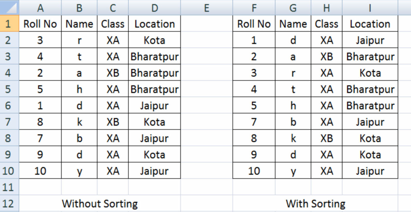
End FunctionSorting the columns using macro (use Range.Sort method)
Sub Sort_Data()
Range("A1:D7”).Sort Key1:=Range("B1"), Order1:=xlAscending, Header:=xlYes
End Sub
Here,
Range: It is refers to the data that you want to sort. Example, A1:D7 Sort: It is the method that will perform sorting operation on the specified range.
Key: It is used to specify the column according to which you want to sort the data. Example, to sort data according to column A, you will use the Key keyword as Key1:=Range(“A1”)
Order: It is used to mentioned the order of sorting, i.e. the ascending or descending order. Example, you will use the Order keyword as Order1:=xlAscending
Header: It is used to specify whether the data set has headers or not. If it has headers, the sorting starts from the second row of the data set, else it starts from the first row. To specify that your data has headers, you will use the Header keyword as Header:=xlYes or xlNo if it does not have headers.
2 thoughts on “Class 10 IT 402 Electronic Spreadsheet (Advanced) – Notes”